
Explaining POWERUP predictions
Source:vignettes/explaining-powerup-predictions.Rmd
explaining-powerup-predictions.RmdPOWERUP uses SHAP values to explain how molecular features contribute to its predictions. For an individual sample, the fitted model prediction can be represented as a baseline value plus the additive contributions of its features. Positive and negative SHAP values move the modeled outcome higher or lower, respectively.
POWERUP provides several complementary views of these explanations. A waterfall plot shows how features contribute to one prediction, a SHAP scatter places those effects in the context of the training cohort, and aggregate contribution plots identify features that contribute most strongly across many samples. Explanation path analysis then asks a different question: whether samples with the same predicted response reach that prediction through recurrent, distinct SHAP patterns.
SHAP values explain the fitted model, not biological causality. A large SHAP contribution means that a feature strongly influenced the model prediction; it does not show that experimentally changing the feature would change the response.
Recreate the example predictions
The first examples use the same compact DepMap Public 26Q1 demonstration data introduced in Get Started with POWERUP. We fit a CTNNB1 dependency model and generate predictions for two held-out samples. See Example data and provenance for details about the bundled data.
expression_path <- system.file("extdata", "powerup_example_gene_expression.csv", package = "powerup")
dependency_path <- system.file("extdata", "powerup_example_gene_dependency.csv", package = "powerup")
user_path <- system.file("extdata", "powerup_example_user_matrix.csv", package = "powerup")

example_expression <- read.csv(expression_path, check.names = FALSE)
example_dependency <- read.csv(dependency_path, check.names = FALSE)
example_user <- read.csv(user_path, check.names = FALSE)

prepared <- prepare_powerup_data(gene_expression = example_expression, response = example_dependency, targets = "CTNNB1", user_matrix = example_user)
models <- fit_powerup_models(prepared, seed = 123L)
models <- add_powerup_predictions(models, prepared)
The two user samples now have both predictions and SHAP contributions that can be examined with the functions below.
Explain an individual prediction
plot_contributions_to_sample() provides the most direct
explanation of an individual POWERUP prediction. The waterfall begins
from the model’s SHAP baseline and shows how the largest feature
contributions move the prediction toward its final value. This baseline
is the constant reference value returned by the fitted XGBoost model
before the sample-specific feature contributions are added.
Here we explain the CTNNB1 dependency predictions for the two held-out samples:
plot_contributions_to_sample(
  models,
  prepared,
  perturbations = "CTNNB1",
  samples = c("ACH-000957", "ACH-002024"),
  source = "user",
  n_features = 6,
  n_columns = 1,
  fixed_axis = TRUE
)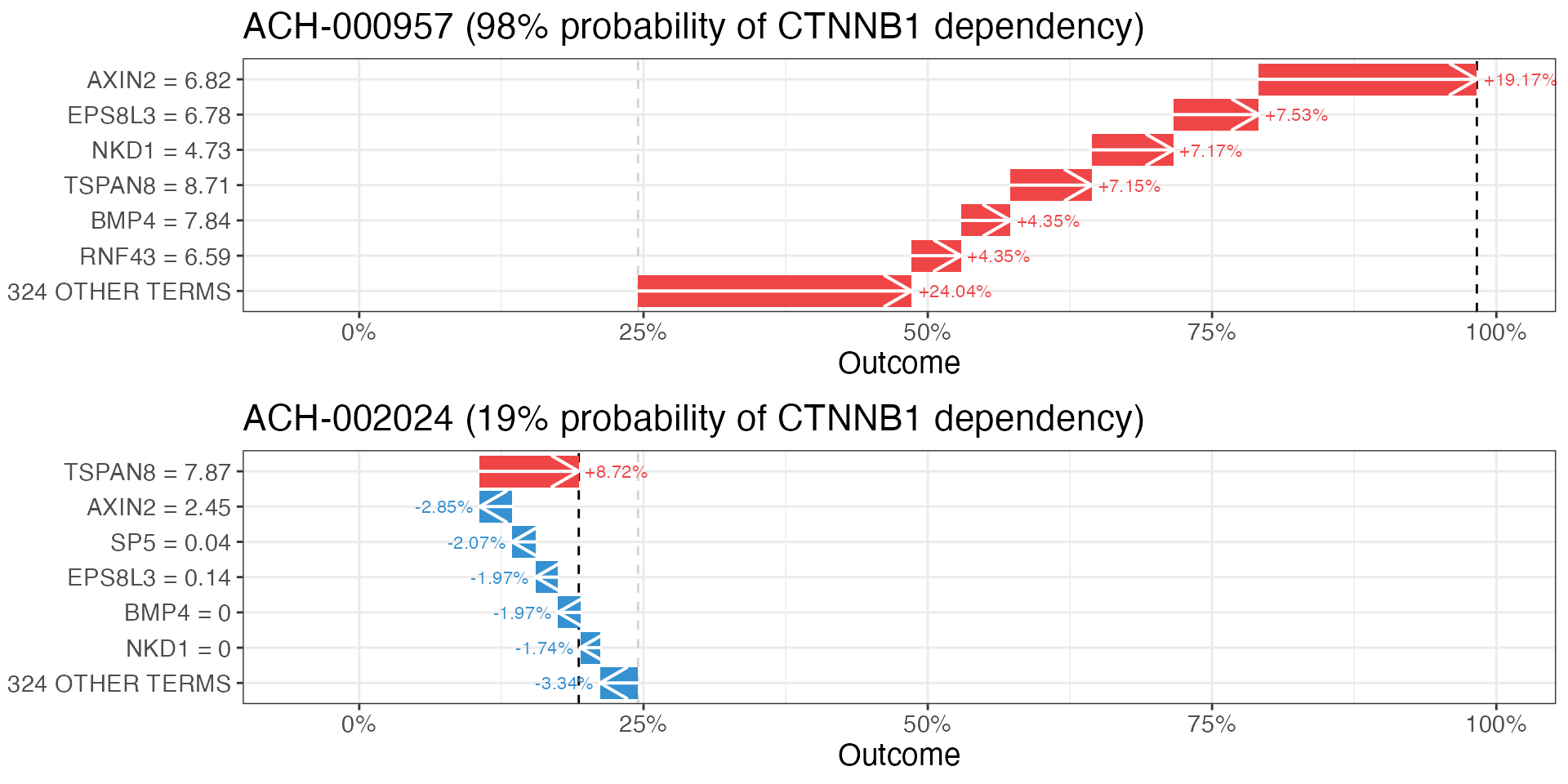
The feature labels also report the corresponding feature values for
the selected sample. n_features controls how many of the
largest absolute SHAP contributions are displayed individually; any
remaining contributions are combined into an “other terms” contribution
so that the displayed contributions still connect the baseline to the
final prediction.
Training samples can be examined in the same way using the default
source = "training". For user samples predicted with
add_powerup_predictions(), use source = "user"
as above.
Notice that the same feature, AXIN2 for example, can have a positive contribution in one sample and a negative contribution in another depending on its expression value. The SHAP contribution shown near each arrow reflects that feature’s influence on the model prediction for that specific sample.
Place a prediction in context
A waterfall shows which features matter for one sample, while
plot_shap_scatter() puts those feature values and SHAP
contributions in the context of all training data.
Each panel plots the feature value on the x-axis against its exact SHAP contribution on the y-axis. Selected training or user samples can then be highlighted on top of this reference distribution to see how they compare.
Here we show the top six CTNNB1 features and overlay the same two user samples:
plot_shap_scatter(
  models,
  prepared,
  perturbation = "CTNNB1",
  n_features = 6,
  samples = c("ACH-000957", "ACH-002024"),
  source = "user",
  sample_colors = c("red", "blue")
)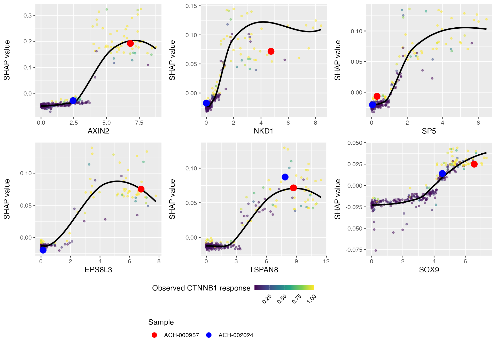
These plots help show how the predictive model evaluates the contribution of a feature across its observed values. The highlighted samples show where an individual prediction falls within that learned relationship.
Because tree-based models can capture nonlinear relationships, the association between a feature value and its SHAP contribution need not be linear or monotonic. Different features can also show different thresholds, plateaus, or changes in direction.
The color of the training points reflects the observed outcome. Samples can therefore have a strong dependency on the target even when one of the displayed features has a low or negative SHAP contribution, and vice versa. This illustrates how the final model prediction reflects the combined contributions of many features rather than any single feature alone.
By default, this function selects the most influential features based
on the training cohort. Specific features can instead be supplied with
the features argument.
Summarize explanations across samples
Local explanations can also be aggregated to identify features that
contribute most strongly across a cohort.
plot_top_contributors() ranks each feature by the sum of
its absolute SHAP contributions across the selected samples.
For the CTNNB1 training cohort:
plot_top_contributors(
  models,
  models_to_use = "CTNNB1",
  data_to_use = "training",
  n_predictors = 10,
  n_columns = 1
)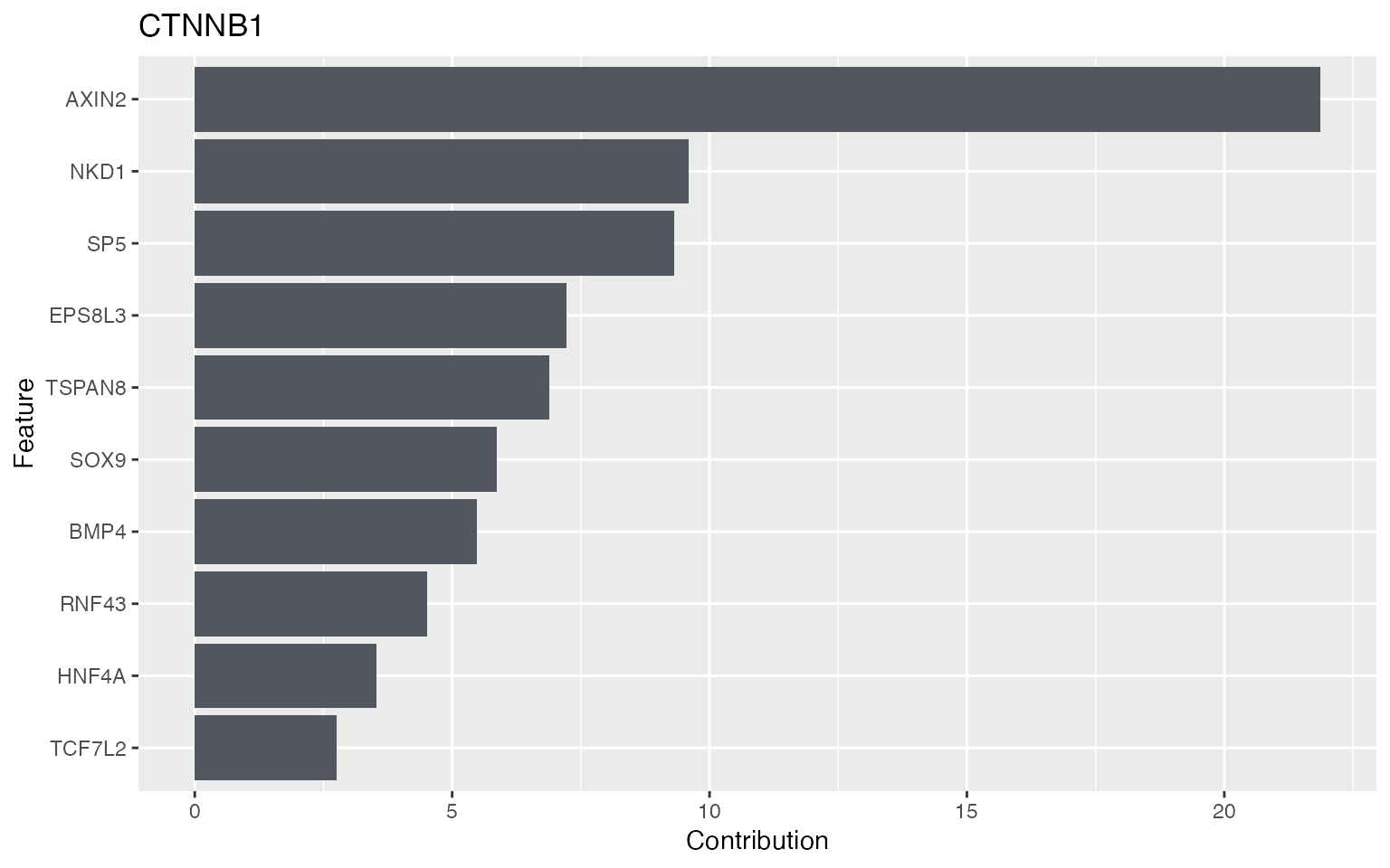
Because the aggregation uses absolute SHAP values, this view measures the overall magnitude of a feature’s influence rather than whether the feature consistently increases or decreases predictions. A feature can therefore rank highly even when its direction differs across samples.
The same summary can be generated for the prediction cohort after
add_powerup_predictions():
plot_top_contributors(
  models,
  models_to_use = "CTNNB1",
  data_to_use = "new_data",
  n_predictors = 10,
  n_columns = 1
)
For analyses containing many fitted models,
summarize_contributions() provides the corresponding
aggregate SHAP values as a model-by-feature matrix for downstream
analysis.
Together, these plots help investigate what drove one prediction, how those effects compare with the reference cohort, and which features matter most across a collection of samples. However, a single aggregate summary can still hide distinct combinations of feature effects that recur among samples with the same predicted response.
Explanation path diversity
POWERUP explanation paths are designed to capture this additional structure. Two samples can receive the same predicted response class (Sensitive or Resistant) while reaching that prediction through different combinations of SHAP contributions (we call these “explanation paths”). Explanation path analysis identifies recurrent SHAP profiles within the predicted Sensitive and Resistant classes and summarizes how many distinct explanation patterns are supported by the training data.
Path discovery is intentionally based on training samples
only. Prediction samples do not define or change the paths.
When the original fitted models contain new predictions,
assign_explanation_paths() can subsequently project those
samples onto the fixed training-defined paths.
For this section, we use the bundled explanation-model object and focus on its CTNNB1 model, which was fitted on a larger reference cohort. This provides more realistic path structure than the compact 300-sample example while keeping file sizes manageable. See Example data and provenance for details about the bundled data.
Load the explanation models
The bundled RDS file retains the training SHAP values and model metadata needed for path analysis. It omits the original expression and response matrices, fitted boosters, uncertainty models, and prediction data.
model_path <- system.file("extdata", "powerup_example_explanation_models.rds", package = "powerup", mustWork = TRUE)
path_models <- readRDS(model_path)

ctnnb1_target <- "ko_ctnnb1"
The bundled object uses POWERUP’s processed perturbation identifier
ko_ctnnb1, while the text of this guide refers to the
corresponding gene symbol CTNNB1 for readability.
Calculate explanation paths
Calculate paths for the CTNNB1 example target:
paths <- calculate_explanation_paths(path_models, targets = ctnnb1_target)
#> Calculating explanation paths: 1 of 1
paths
#> $results
#> $results$ko_ctnnb1
#> $results$ko_ctnnb1$target
#> [1] "ko_ctnnb1"
#>
#> $results$ko_ctnnb1$class_summary
#> # A tibble: 2 × 42
#> target mean_r prediction_class n_cell_lines eligible_for_multipath
#> <chr> <dbl> <chr> <int> <lgl>
#> 1 ko_ctnnb1 0.740 Sensitive 119 TRUE
#> 2 ko_ctnnb1 0.740 Resistant 1021 TRUE
#> # ℹ 37 more variables: n_supported_cell_lines <int>,
#> # supported_cell_line_fraction <dbl>, n_outlier_cell_lines <int>,
#> # outlier_fraction <dbl>, selected_raw_cluster_count <int>,
#> # selected_path_count <int>, effective_path_count <dbl>,
#> # dominant_path_fraction <dbl>, dominant_path_fraction_of_class <dbl>,
#> # path_entropy <dbl>, path_evenness <dbl>, silhouette_score <dbl>,
#> # mean_pairwise_distance <dbl>, median_pairwise_distance <dbl>, …
#>
#> $results$ko_ctnnb1$path_summary
#> # A tibble: 5 × 11
#> prediction_class explanation_path_id n_cell_lines fraction_of_supported
#> <chr> <int> <int> <dbl>
#> 1 Sensitive 1 89 0.817
#> 2 Sensitive 2 20 0.183
#> 3 Resistant 1 776 0.872
#> 4 Resistant 2 62 0.0697
#> 5 Resistant 3 52 0.0584
#> # ℹ 7 more variables: mean_prediction <dbl>, median_prediction <dbl>,
#> # min_prediction <dbl>, max_prediction <dbl>, predominant_features <chr>,
#> # distinguishing_features <chr>, fraction_of_class <dbl>
#>
#> $results$ko_ctnnb1$assignments
#> # A tibble: 1,140 × 8
#> target matrix_row_index sample prediction_class reconstructed_predic…¹
#> <chr> <int> <chr> <chr> <dbl>
#> 1 ko_ctnnb1 5 ACH-000461 Sensitive 0.932
#> 2 ko_ctnnb1 7 ACH-002023 Sensitive 0.943
#> 3 ko_ctnnb1 12 ACH-001098 Sensitive 0.805
#> 4 ko_ctnnb1 15 ACH-000769 Sensitive 0.892
#> 5 ko_ctnnb1 16 ACH-000421 Sensitive 0.699
#> 6 ko_ctnnb1 33 ACH-000138 Sensitive 0.547
#> 7 ko_ctnnb1 54 ACH-001991 Sensitive 0.849
#> 8 ko_ctnnb1 73 ACH-000880 Sensitive 0.900
#> 9 ko_ctnnb1 76 ACH-000552 Sensitive 0.957
#> 10 ko_ctnnb1 78 ACH-000222 Sensitive 0.768
#> # ℹ 1,130 more rows
#> # ℹ abbreviated name: ¹reconstructed_prediction
#> # ℹ 3 more variables: explanation_path_id <int>, is_outlier <lgl>,
#> # assignment_type <chr>
#>
#> $results$ko_ctnnb1$diagnostics
#> # A tibble: 2 × 15
#> prediction_class dendrogram_cut_height actual_raw_cluster_count
#> <chr> <dbl> <int>
#> 1 Sensitive 0.7 6
#> 2 Resistant 0.7 11
#> # ℹ 12 more variables: raw_cluster_sizes_descending <chr>,
#> # min_supported_path_size_required <dbl>, n_supported_paths <int>,
#> # supported_path_sizes_descending <chr>, n_supported_cell_lines <int>,
#> # supported_cell_line_fraction <dbl>, n_outlier_clusters <int>,
#> # n_outlier_cell_lines <int>, outlier_fraction <dbl>, silhouette_score <dbl>,
#> # selection_reason <chr>, target <chr>
#>
#> $results$ko_ctnnb1$feature_summary
#> # A tibble: 105 × 7
#> prediction_class explanation_path_id n_cell_lines_in_path feature mean_shap
#> <chr> <int> <int> <chr> <dbl>
#> 1 Sensitive 1 89 axin2 0.178
#> 2 Sensitive 1 89 bmp4 0.0536
#> 3 Sensitive 1 89 rnf43 0.0473
#> 4 Sensitive 1 89 nkd1 0.0295
#> 5 Sensitive 1 89 krba1 0.0204
#> 6 Sensitive 1 89 bcl2l15 0.0183
#> 7 Sensitive 1 89 eps8l3 0.0178
#> 8 Sensitive 1 89 gpr35 0.0164
#> 9 Sensitive 1 89 cdx2 0.0110
#> 10 Sensitive 1 89 hnf4a 0.00990
#> # ℹ 95 more rows
#> # ℹ 2 more variables: mean_abs_shap <dbl>,
#> # mean_shap_difference_vs_other_paths <dbl>
#>
#>
#>
#> $errors
#> # A tibble: 0 × 0
#>
#> $parameters
#> $parameters$min_mean_r
#> NULL
#>
#> $parameters$response_cutoff
#> NULL
#>
#> $parameters$dendrogram_cut_height
#> [1] 0.7
#>
#> $parameters$min_path_size
#> [1] 10
#>
#> $parameters$min_path_fraction
#> [1] 0.05
#>
#> $parameters$driver_thresholds
#> [1] 0.5 0.7 0.9
#>
#> $parameters$top_n_features
#> [1] 10
#>
#> $parameters$distance
#> [1] "correlation"
#>
#> $parameters$source
#> [1] "training_shap"
#>
#>
#> attr(,"class")
#> [1] "powerup_explanation_paths" "list"Note: Using targets = NULL, the default, analyzes every
eligible target in the supplied model object:
Within each predicted response class, POWERUP represents training samples in a common space of named SHAP features, calculates SHAP-profile distance, and performs average-linkage hierarchical clustering. Sensitive and Resistant samples are analyzed separately, so a sample predicted to be Sensitive will not cluster with Resistant training samples.
The default path-definition settings are:
| Setting | Default |
|---|---|
| Dendrogram cut height | 0.70 |
| Minimum path size | 10 training samples |
| Minimum path fraction | 5% of the prediction class |
| SHAP-profile distance | Correlation |
| Linkage | Average |
Each response class is represented by one average-linkage dendrogram, which is cut once at the specified height. A supported path must contain at least the larger of the minimum path size and the minimum class fraction. Branches below that support threshold are labeled as outliers rather than used to define additional paths. If no branch from the fixed-height cut satisfies the support threshold, the prediction class falls back to a single explanation path.
The dendrogram cut alone defines the paths: POWERUP does not scan
candidate path counts or use silhouette or subsampling stability to
choose, reject, or tune the solution. After the supported path
assignments have been fixed, silhouette_score is calculated
as a descriptive measure of path separation when the class contains at
least two supported paths; it is NA for a single-path
class.
Please note that a class with fewer than twice the minimum path size
cannot contain two paths that each satisfy that minimum. For example, a
perturbation with only 15 sensitive cell lines cannot support two
distinct explanation paths at 10 samples per path minimum. POWERUP
retains these classes but marks them with
eligible_for_multipath = FALSE.
Visualize explanation paths for one target
plot_explanation_paths() helps us visualize the
supported paths for one target:
ctnnb1_plot <- plot_explanation_paths(paths, target = ctnnb1_target, models = path_models, top_n = 10)
ctnnb1_plot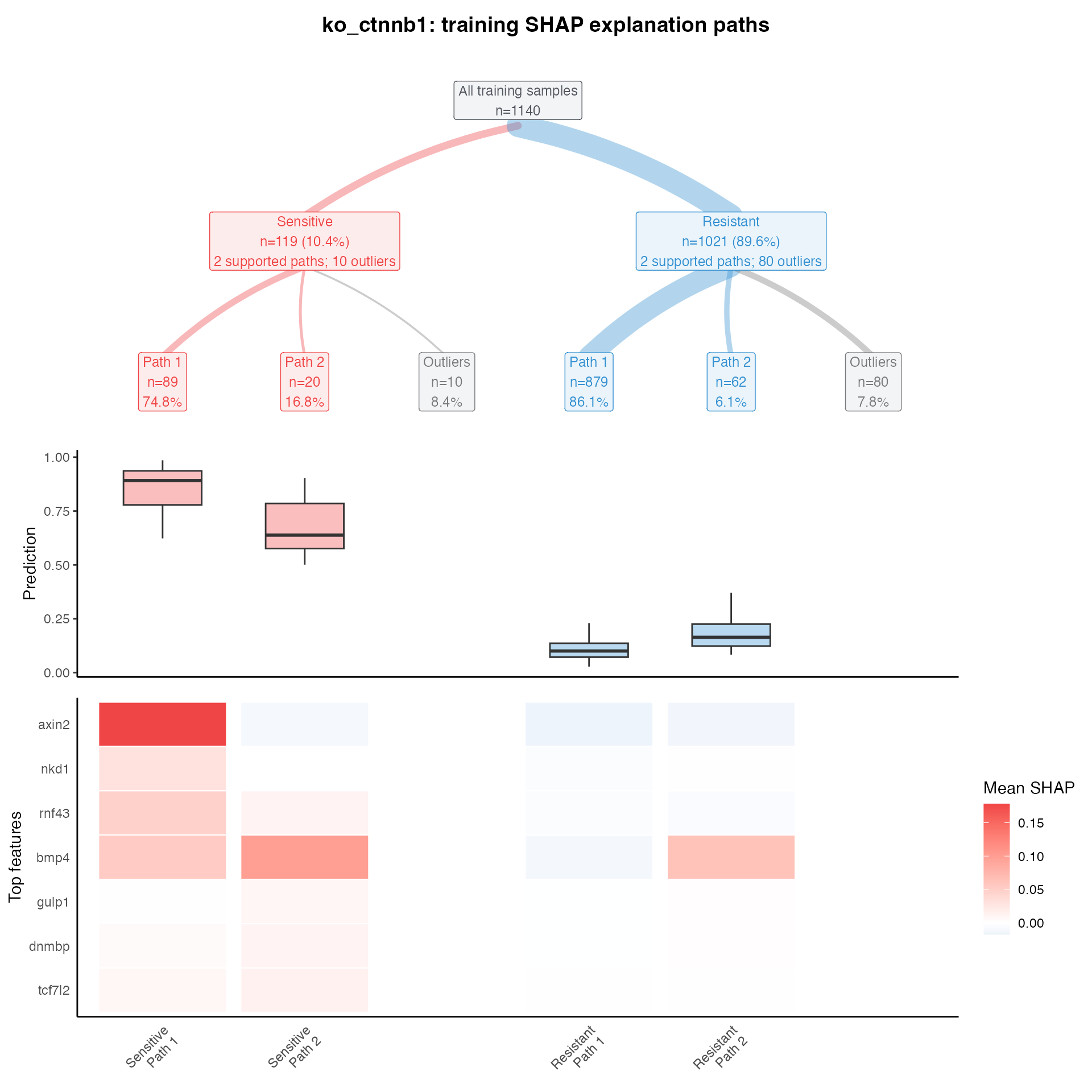
The figure combines three views of the explanations: the Sensitive and Resistant path hierarchy, the distribution of model predictions within each supported path, and a signed mean-SHAP heatmap showing features that characterize those paths.
By default, the heatmap features are statistical path markers. For each path, POWERUP compares per-sample SHAP values with the other supported paths in the same response class using a Wilcoxon rank-sum test, followed by Benjamini-Hochberg correction. The default marker filters require an adjusted p-value of 0.05 or less, an absolute mean-SHAP difference of at least 0.005, and a nonzero SHAP value in at least half of one comparison group. Positive markers are shown by default. When a response class contains only one supported path, there is no path-vs-path comparison, so its displayed features fall back to those with the largest mean absolute SHAP values.
Notice that in the case of CTNNB1, the Sensitive class supports two distinct explanation paths: one with high AXIN2 SHAP, a classic biomarker of activated Wnt signaling, and one where BMP4 is more dominant.
The complete marker statistics are attached to the returned plot:
ctnnb1_markers <- attr(ctnnb1_plot, "path_markers")
head(ctnnb1_markers)
#> # A tibble: 6 × 16
#>   prediction_class explanation_path_id feature path_mean_shap
#>   <chr>                          <int> <chr>            <dbl>
#> 1 Sensitive                          1 a1bg        -0.0000171
#> 2 Sensitive                          1 aadat        0.000192
#> 3 Sensitive                          1 abca2        0
#> 4 Sensitive                          1 abhd17c      0
#> 5 Sensitive                          1 abhd2        0.00165
#> 6 Sensitive                          1 ache         0.000215
#> # ℹ 12 more variables: other_paths_mean_shap <dbl>, mean_shap_difference <dbl>,
#> #   absolute_mean_shap_difference <dbl>, path_nonzero_fraction <dbl>,
#> #   other_paths_nonzero_fraction <dbl>, maximum_nonzero_fraction <dbl>,
#> #   wilcoxon_u <dbl>, common_language_probability <dbl>,
#> #   rank_biserial_correlation <dbl>, absolute_rank_biserial_correlation <dbl>,
#> #   p_value <dbl>, adjusted_p_value <dbl>
Note for large POWERUP jobs
In large runs, saving the fitted model objects can be resource-intensive. If the original fitted model object is unavailable, the plot can instead use the predominant features already stored during path calculation:
plot_explanation_paths(paths, target = ctnnb1_target, feature_selection = "mean_absolute_shap")Summarize explanation diversity
summarize_explanation_paths() reduces the detailed path
object to class-level and path-level tables:
path_summary <- summarize_explanation_paths(paths)per_class contains one row for each target and predicted
response class. A compact set of the most useful fields is:
path_summary$per_class[, c(
  "target",
  "prediction_class",
  "n_cell_lines",
  "eligible_for_multipath",
  "dendrogram_cut_height",
  "selected_path_count",
  "effective_path_count",
  "silhouette_score",
  "dominant_path_fraction",
  "top_driver_feature",
  "n_features_50pct"
)]
#> # A tibble: 2 × 11
#>   target    prediction_class n_cell_lines eligible_for_multipath
#>   <chr>     <chr>                   <int> <lgl>
#> 1 ko_ctnnb1 Sensitive                 119 TRUE
#> 2 ko_ctnnb1 Resistant                1021 TRUE
#> # ℹ 7 more variables: dendrogram_cut_height <dbl>, selected_path_count <int>,
#> #   effective_path_count <dbl>, silhouette_score <dbl>,
#> #   dominant_path_fraction <dbl>, top_driver_feature <chr>,
#> #   n_features_50pct <int>
dendrogram_cut_height records the height used to define
the paths. selected_path_count is the number of supported
paths retained after the fixed-height cut and minimum-support rule.
effective_path_count additionally reflects how evenly
samples are distributed among those paths, while
dominant_path_fraction reports the fraction of supported
samples belonging to the largest path. silhouette_score
describes the separation of the resulting supported paths after
assignment and is not used to select the path solution.
top_driver_feature identifies the feature contributing
most strongly to overall between-path SHAP separation.
n_features_50pct reports the minimum number of features
required to account for 50% of the between-path SHAP dispersion.
per_path contains one row for each supported path. It
reports the path size and prediction distribution together with two
complementary feature summaries:
-
predominant_featuresare features with the largest absolute mean SHAP values within that path. -
distinguishing_featuresare features with the largest signed mean-SHAP differences between that path and the other supported paths in the same response class.
For CTNNB1:
path_summary$per_path[
  path_summary$per_path$target == ctnnb1_target,
  c(
    "target",
    "prediction_class",
    "explanation_path_id",
    "n_cell_lines",
    "fraction_of_class",
    "mean_prediction",
    "predominant_features",
    "distinguishing_features"
  )
]
#> # A tibble: 5 × 8
#>   target    prediction_class explanation_path_id n_cell_lines fraction_of_class
#>   <chr>     <chr>                          <int>        <int>             <dbl>
#> 1 ko_ctnnb1 Sensitive                          1           89            0.748
#> 2 ko_ctnnb1 Sensitive                          2           20            0.168
#> 3 ko_ctnnb1 Resistant                          1          776            0.760
#> 4 ko_ctnnb1 Resistant                          2           62            0.0607
#> 5 ko_ctnnb1 Resistant                          3           52            0.0509
#> # ℹ 3 more variables: mean_prediction <dbl>, predominant_features <chr>,
#> #   distinguishing_features <chr>
The descriptive distinguishing_features and the
statistical markers used by plot_explanation_paths() answer
related but different questions. The former rank features by the
magnitude of between-path mean-SHAP differences, whereas the latter
additionally require the per-sample SHAP distributions to pass
statistical and effect-size filters.
Inspect training-sample path assignments
The full paths object retains the training-sample
assignments used to construct the summaries. These can be helpful for
further investigation into the identity of samples clustering to
different paths. Retrieve them with
get_explanation_path_assignments():
ctnnb1_assignments <- get_explanation_path_assignments(paths, target = ctnnb1_target)
head(ctnnb1_assignments)
#> # A tibble: 6 × 8
#> target matrix_row_index sample prediction_class reconstructed_predict…¹
#> <chr> <int> <chr> <chr> <dbl>
#> 1 ko_ctnnb1 5 ACH-000461 Sensitive 0.932
#> 2 ko_ctnnb1 7 ACH-002023 Sensitive 0.943
#> 3 ko_ctnnb1 12 ACH-001098 Sensitive 0.805
#> 4 ko_ctnnb1 15 ACH-000769 Sensitive 0.892
#> 5 ko_ctnnb1 16 ACH-000421 Sensitive 0.699
#> 6 ko_ctnnb1 33 ACH-000138 Sensitive 0.547
#> # ℹ abbreviated name: ¹reconstructed_prediction
#> # ℹ 3 more variables: explanation_path_id <int>, is_outlier <lgl>,
#> # assignment_type <chr>Supported paths are numbered separately within each prediction class.
Samples assigned to undersized branches that are retained as outliers
have explanation_path_id = 0.
A simple count of the CTNNB1 assignments is:
with(ctnnb1_assignments, table(prediction_class, explanation_path_id, useNA = "ifany"))
#>                 explanation_path_id
#> prediction_class   0   1   2   3
#>        Resistant 131 776  62  52
#>        Sensitive  10  89  20   0
Calling get_explanation_path_assignments(paths) without
a target returns assignments for every analyzed target.
When new prediction samples are available in the original fitted
models, assign_explanation_paths() assigns each sample to
its closest supported training path within the same predicted response
class. These assignments are descriptive similarities to fixed
training-derived paths; the prediction samples never redefine the path
structure.
Interpreting SHAP explanations
The explanation functions in POWERUP operate at different levels but describe the same fitted predictive model. Waterfalls explain individual predictions, SHAP scatters place individual effects within the reference cohort, aggregate contributions summarize recurring model influence across samples, and explanation paths identify recurrent multifeature SHAP patterns within predicted response classes.
None of these analyses establishes that a feature is a causal regulator of the measured response. Explanation paths should likewise not be interpreted automatically as biological subtypes. Their value is in identifying reproducible structures in how the model arrives at its predictions, which can then be considered alongside model performance, prediction uncertainty, experimental evidence, and biological context.
For guidance on prediction uncertainty and other model outputs, see Interpreting POWERUP results. To incorporate experimental measurements into POWERUP priors, continue with Experimental observations and posterior updating.
References
To learn more about the general SHAP framework and its theoretical foundation, see:
Lundberg, S.M. and Lee, S.-I. A Unified Approach to Interpreting Model Predictions. Advances in Neural Information Processing Systems 30 (2017). https://papers.nips.cc/paper/7062-a-unified-approach-to-interpreting-model-predictions
For tree-based models and the TreeSHAP framework used to interpret tree ensembles such as XGBoost, see:
Lundberg, S.M., Erion, G., Chen, H. et al. From local explanations to global understanding with explainable AI for trees. Nature Machine Intelligence 2, 56-67 (2020). https://doi.org/10.1038/s42256-019-0138-9
Session information
sessionInfo()
#> R version 4.4.2 (2024-10-31)
#> Platform: aarch64-apple-darwin20
#> Running under: macOS Sequoia 15.7.3
#>
#> Matrix products: default
#> BLAS:   /Library/Frameworks/R.framework/Versions/4.4-arm64/Resources/lib/libRblas.0.dylib
#> LAPACK: /Library/Frameworks/R.framework/Versions/4.4-arm64/Resources/lib/libRlapack.dylib;  LAPACK version 3.12.0
#>
#> locale:
#> [1] en_US.UTF-8/en_US.UTF-8/en_US.UTF-8/C/en_US.UTF-8/en_US.UTF-8
#>
#> time zone: America/New_York
#> tzcode source: internal
#>
#> attached base packages:
#> [1] stats     graphics  grDevices utils     datasets  methods   base
#>
#> other attached packages:
#> [1] powerup_1.0.117
#>
#> loaded via a namespace (and not attached):
#>  [1] utf8_1.2.4        sass_0.4.9        future_1.34.0     generics_0.1.3
#>  [5] tidyr_1.3.1       stringi_1.8.4     lattice_0.22-6    listenv_0.9.1
#>  [9] digest_0.6.37     magrittr_2.0.3    evaluate_1.0.3    grid_4.4.2
#> [13] fastmap_1.2.0     xgboost_3.2.1.1   jsonlite_2.0.0    Matrix_1.7-3
#> [17] mgcv_1.9-1        purrr_1.1.0       viridisLite_0.4.2 scales_1.3.0
#> [21] codetools_0.2-20  textshaping_1.0.0 jquerylib_0.1.4   cli_3.6.5
#> [25] rlang_1.1.6       parallelly_1.42.0 splines_4.4.2     cowplot_1.1.3
#> [29] munsell_0.5.1     withr_3.0.2       cachem_1.1.0      yaml_2.3.10
#> [33] tools_4.4.2       parallel_4.4.2    dplyr_1.1.4       colorspace_2.1-1
#> [37] ggplot2_3.5.1     rsample_1.2.1     globals_0.16.3    vctrs_0.6.5
#> [41] R6_2.6.1          lifecycle_1.0.4   stringr_1.5.2     fs_1.6.5
#> [45] htmlwidgets_1.6.4 ragg_1.5.1        furrr_0.3.1       pkgconfig_2.0.3
#> [49] desc_1.4.3        gtable_0.3.6      pkgdown_2.2.0     pillar_1.10.1
#> [53] bslib_0.9.0       glue_1.8.0        data.table_1.17.0 systemfonts_1.2.2
#> [57] xfun_0.51         tibble_3.3.0      tidyselect_1.2.1  knitr_1.50
#> [61] farver_2.1.2      nlme_3.1-167      htmltools_0.5.8.1 labeling_0.4.3
#> [65] rmarkdown_2.29    compiler_4.4.2